Heads up; its more fun to read this blog post if you have seen directed acyclic graphs (DAGs) before, as this blog post won’t provide an introduction to DAGs.
When I started to read up on causal inference during the beginning of my PhD studies, I often got stuck on the assumption of exchanability, i.e., Rubin’s ignorability assumption: \(Y^x \perp\!\!\!\!\perp X | Z\). I understood what the assumption means in theory and I understood how to use DAGs to identify confounders and colliders. Intuitively, I understood how the ignorability assumption and DAGs are connected, but I did not understand how they are theoretically connected. I mean, there are usually no counterfactuals in a DAG so how can one use DAGs to reason about whether counterfactuals are independent of the treatment assignment \(X\). One solution is to use singe world interventions graphs (SWIGs), but they never felt really natural to me. Pearl’s do-calculus instead offers a very nice combination of DAGs and the ignorability in my opinion. Hence, I think it is worth taking a closer look at the rules of do-calculus and how they combine the irgnorability assumption and DAGs.
Before we can dive into Pearl’s do-calculus and look at some examples, we first need to introduce a bit of specific notation. First, let \(W\), \(X\), \(Y\), and \(Z\) be a set of unique variables. Second, let \(G\) be a directed acyclic graph which is associated with a causal model, let \(G_\overline{X}\) be a submodel of \(G\) in which we remove all arrows going into \(X\), and let \(G_\underline{X}\) be a submodel of \(G\) in which we remove all arrows going out of \(X\). Third, let \(\text{do}(x)\) define an operator for intervening on \(x\). For example, \(P(y|\text{do}(x'))\) indicates the value of \(y\) if we would change the value of \(x\) to the value \(x'\). Lastly, let \(X \perp\!\!\!\!\perp Y\) denote that \(X\) and \(Y\) are independent of each other.
In his book Causality, Pearl defines the three rules of do-calculus which can be used to identify causal effects with the help of DAGs. The overall aim of do-calculus is to translate expression including do-statements to expression only including observed data. This allows us to identify and later estimate a causal effect using our observed data. Put in other word, using do-calculus, we can translate a causal expression into an expression only including associations which we then can estimate from our observed data. This allows us to interpret association as causation if certain assumptions are fulfilled. Something that previously was only allowed the devil of epidemiological research.
Now you’re ready for the three rules. Listing carefully.
Rule 1 (Insertion/deletion of observations) \[ P(y|\text{do}(x), z, w) = P(y|\text{do}(x), w) \text{ if } Y \perp\!\!\!\!\perp Z|X,W \text{ in } G_{\overline{X}} \]
In words, this tells us that we can remove a variable \(z\) from our expression if \(z\) is independent of \(y\), given \(x\) and potentially other variables \(w\), in the DAG in which we remove all arrows going into \(x\).
Rule 2 (Action/observation exchange) \[ P(y|\text{do}(x), \text{do}(z), w) = P(y|\text{do}(x), z, w) \text{ if } Y \perp\!\!\!\!\perp Z|X,W \text{ in } G_{\overline{X}, \underline{Z}} \]
In word, this tells us that we can replace the action \(do(z)\) with the variable \(z\) observed in the data if \(y\) and \(z\) are independent, given \(x\) and potentially other variables \(w\), in the DAG in which we remove the arrow going into \(x\) and out of \(z\). Note that this rule is a generalisation of the back-door criteria which you might now from before. If we are only interested in one action, e.g., \(\text{do}(x)\) we can simplify rule 2 as follow:
\[ P(y|\text{do}(x), w) = P(y|x, w) \text{ if } Y \perp\!\!\!\!\perp X|W \text{ in } G_{\underline{X}} \] This now is pretty much an expression of the commonly known back-door criteria.
Rule 3 (insertion/deletion of actions) \[ P(y|\text{do}(x), \text{do}(z), w) = P(y|\text{do}(x), w) \text{ if } Y \perp\!\!\!\!\perp Z|X, W \text{ in } G_{\overline{X}, \overline{Z(W)}} \]
where \(Z(W)\) is the set of \(Z\)-nodes that are not ancestors of any \(W\)-node in \(G_\overline{X}\).
Last but not least, rule 3 is probably the most complicated one. In words rule 3 tells us that we can remove an expression, e.g., \(\text{do}(y)\) from our expression if \(Y\) and \(Z\) are independent, given \(X\) and potentially other variables \(Z\), in the graph were we remove all arrow going out of \(X\) and all nodes of \(Z\) that are not ancestors of \(W\).
Let’s use these rules of do-calculus for identifying causal effects in some example graphs.
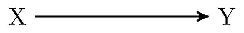
The first example in Figure 1 (a) might seem trivial, but I thought it might be a smooth start. In this graph there are no arrows connecting \(X\) and \(Y\) in \(G_\underline{X}\), that is, if we remove all the arrows going out of \(X\). Hence, \(X\) and \(Y\) are independent in \(G_\underline{X}\), which means that we can apply rule 2 of do-calculus:
\[ P(y|\text{do}(x)) = P(y|x) \]
Success! Using do-calculus we could replace all the do-statements with observed variables, which now allows us to estimate the causal effect of changing \(X\) on \(Y\) based on our observed data. This was quite an easy example. But before we continue with the next example, let’s take a closer look at \(G_\underline{X}\) again. The reason why we are interested in looking at the graph in which we remove all arrows going out from \(X\) is that we want to make sure that \(X\) is only affecting \(Y\) directly or through causes that are caused by \(X\), i.e., we are interested in the total effect of \(X\) on \(Y\). Thus, if we remove all arrows going out of \(X\) or going into \(Y\), and we find that in this submodel there is no open causal path between \(X\) and \(Y\), we can be sure, that in the whole model \(G\), all causal paths between \(X\) and \(Y\) must be direct paths, i.e., paths that we want to include in our estimation.
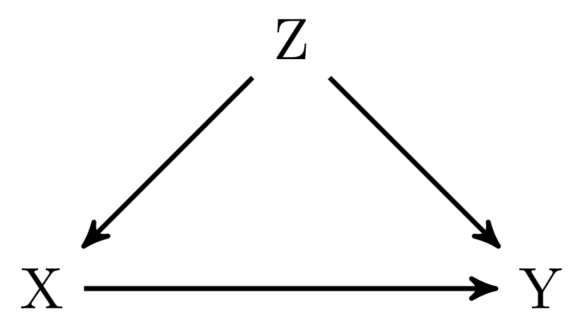
Figure 1 (b) includes a classical example of confounding, in which the variable \(Z\) confounds the effect of \(X\) on \(Y\). If we remove all arrows going out of \(X\), we find that \(X\) is still associated with \(Y\) through the fork \(X \leftarrow Z \rightarrow Y\). Hence, we cannot directly disentangle the direct effect of \(X\) on \(Y\) and the association between \(X\) and \(Y\) that is due to the confounding of \(Z\). However, as stated in rule 2 we can also condition on other variables to render \(X\) and \(Y\) independent in \(G_\underline{X}\).
\[ \begin{align} P(y|\text{do}(x)) & = \sum_z P(y|\text{do}(x), z) P(z) \\ & = \sum_z P(y|x, z) P(z) && \text{Rule 2: } Y \perp\!\!\!\!\perp X|Z \text{ in } G_{\underline{X}} \\ \end{align} \]
Ok, let’s go through this in more detail. The first step we need to do is to condition our analysis on the variable \(Z\). This renders \(X\) and \(Y\) independent in \(G_\underline{X}\). After this, we can now replace \(P(y|\text{do}(x), z)\) with \(P(y|x, z)\) as \(X\) and \(Y\) are independent when conditioning on \(Z\).
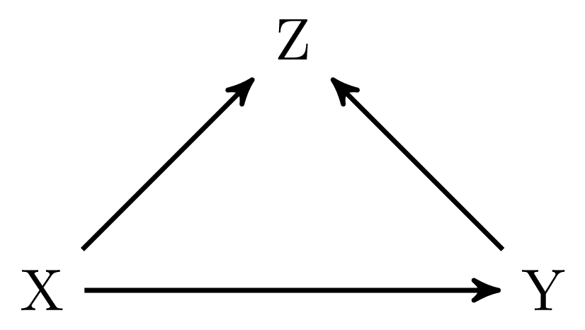
Figure 1 (c) again is a more simple example. In this graph \(X\) and \(Y\) are independent in \(G_\underline{X}\) because \(Z\) is a collider on the path \(X \rightarrow Z \leftarrow Y\). Hence, we can just calculate \(P(y|\text{do}(x))\) based on our observed data \(P(y|x)\).
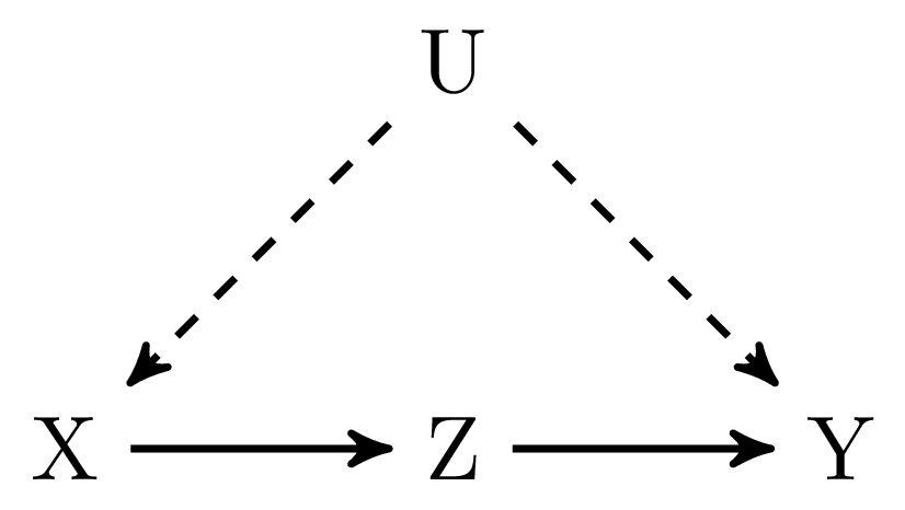
Figure 1 (d) is a tricky one and in contrast to the graphs before, we cannot only rely on rule 2 in order to identify the causal effect of \(X\) on \(Y\). Using only the back-door criteria would not allow us to identify the causal effect of \(X\) on \(Y\) in this graph, but using do-calculus we actually can identify this effect. For this, let’s first take a look at the effect that we would like to estimate:
\[ P(y|\text{do}(x)) = \sum_z P(y|\text{do}(x), z) P(z|x) \tag{1}\]
Unfortunately, we cannot estimate the first part of the right hand hand side directly using only observed data, but we can achieve this with the help of both rule 2 and 3.
\[ \begin{align} P(y|\text{do}(x), z) & = P(y|\text{do}(x), \text{do}(y)) && \text{Rule 2: } Y \perp\!\!\!\!\perp Z \text{ in } G_{\overline{X}\underline{Z}} \\ & = P(y| \text{do}(y)) && \text{Rule 3: } Y \perp\!\!\!\!\perp X \text{ in } G_{\overline{X}\overline{Z}} \\ & = \sum_x P(y| x, z) P(x) && \text{Rule 2: } Y \perp\!\!\!\!\perp Z |X \text{ in } G_{\underline{Z}} \end{align} \tag{2}\]
Now, we yielded an expression for the first part of the right hand site that only includes observed variables. Let’s do the same for the second part of the right hand side in Equation 1. Translating this part of the equation to an expression, only including observed variables, is actually a lot easier, as \(Y\) is a collider on the path \(X \leftarrow U \rightarrow Y \leftarrow Z\) which renders Z and Y independent in \(G_\underline{X}\).
\[ \begin{align} P(z|\text{do}(x)) = P(z|x) && \text{Rule 2: } Z \perp\!\!\!\!\perp X \text{ in } G_{\underline{X}} \end{align} \tag{3}\]
Now, we have all pieces that we need in order to translate Equation 1 into an expression only including observed variables. Let’s substitute Equation 1 with Equation 2 and Equation 3:
\[ P(y|\text{do}(x)) = \sum_z P(z|x) \sum_{x'} P(y| x', z) P(x') \tag{4}\]
Please note that we used \(x'\) in Equation 4 in order to differentiate between the \(x\) in \(\text{do}(x)\) and the \(x\) observed in our dataset. The second part of Equation 4 means a summation over all observed values of \(X\) independent of the value that is chosen for \(\text{do}(x)\).
By the way, if you don’t want to buy Pearl’s causality book, but you’re still interested in reading more about do-calculus, you can find a short introduction to do-calculus by Pearl here. This paper also links to some other interesting applications of do-calculus including, e.g., selection bias and transportability analysis..